
Tutorial: QM/MM Simulation of a Chromophore–Solvent System through the Q-Chem/Amber Interface
Yuezhi Mao, Department of Chemistry and Biochemistry, San Diego State University
In this tutorial, we demonstrate how to perform an excited-state QM/MM simulation for 2-(2’-pyridyl)benzimidazole (PBI, Figure 1) in methanol solvent using the Q-Chem/Amber interface. The tutorial consists of two sections: (i) setting up the simulation box and generating an equilibrium ground-state ensemble; (ii) setting up and running excited-state QM/MM simulations for studying ultrafast excited-state proton transfer (ESPT). Note that part (i) does not require Q-Chem; it is included to make the tutorial self-contained.

Figure 1. The PBI molecule
Part I: Generating a ground-state ensemble for the PBI-methanol system
Before starting, ensure that the Amber script (typically named “amber.sh” under the main Amber directory) is loaded. We then need to generate the General Amber Force Field (GAFF) parameters for the solute and solvent molecules. This can be done by following the steps below (using PBI as an example):
- Optimize the geometry of PBI using a routine method (e.g., B3LYP-D3(BJ)/def2-SVPD). Open the optimized geometry using IQmol and save it as a PDB file (PBI_iqmol.pdb)
- Make the PDB file fully compatible with Amber:
pdb4amber -i PBI_iqmol.pdb -o PBI.pdb - Change the residue name from “UNL” to “PBI”
- Use antechamber to generate the GAFF parameters:
antechamber -i PBI.pdb -fi pdb -o PBI.mol2 -fo mol2 -c bcc -s 2 -rn PBI
Then identify if any force field parameters are missing and write them to the .frcmod file:parmchk2 -i PBI.mol2 -f mol2 -o PBI.frcmod
Here the semi-empirical AM1-BCC method (specified by“-c bcc”) is used to determine the atomic charges. Alternatively, one can use the “RESP” charges, which requires a simple electronic structure calculation at the HF/6-31G(d) level. The user is referred to the Amber manual regarding the procedure to obtain RESP charges. - Repeat the same procedure for methanol. Use residue name “MNL”. Ensure that the following files are prepared:
methanol.pdb methanol.mol2 methanol.frcmod
We will then use Packmol to build the simulation box. Below is a Packmol script (named as “packmol_40A.inp”) to generate a 40 Å × 40 Å × 40 Å box:
tolerance 2.0

filetype pdb

output PBI_958methanol_40A.pdb

#one PBI at the center

structure PBI.pdb

  number 1

  center

  fixed 0. 0. 0. 0. 0. 0.

end structure

#methanol (density 0.792 g/ml)

structure methanol.pdb

  number 958

  inside cube -20. -20. -20. 40. #from -20 to 20 in each direction

end structure
It is determined that 958 methanol molecules are needed to match the bulk density 0.792 g/mL. One can then execute the Packmol script with:
packmol < packmol_40A.inp
to generate the simulation box represented by “PBI_958methanol_40A.pdb”.
Finally, we will use the TLeap program to prepare the input coordinate and topology files needed for Amber simulation. The tleap script (named as “tleap_40A.in”):
source leaprc.gaff

MNL = loadmol2 methanol.mol2

PBI = loadmol2 PBI.mol2

PBIbox = loadpdb PBI_958methanol_40A.pdb

loadamberparams methanol.frcmod

loadamberparams PBI.frcmod

setbox PBIbox centers

saveAmberParm PBIbox PBI_958methanol_40A.prmtop PBI_958methanol_40A.inpcrd

quit
Executing the tleap script generates the input coordinate (.inpcrd) and topology (.prmtop) files.
We are now ready to perform classical MD simulations using GAFF. The following procedure largely follows the Amber tutorial “Simple Simulation of Alanine Dipeptide”, where detailed explanations of the Amber input keywords are provided. These simulations can be carried out using the sander.MPI program if AmberTools was compiled with MPI enabled.
Energy minimization (1500 steepest descent + 1500 conjugate gradient steps):
mpirun -np 16 sander.MPI -O -i 01_Min.in -o 01_Min.out -p PBI_958methanol_40A.prmtop -c PBI_958methanol_40A.inpcrd -r min.rst &
where the Amber input file 01_Min.in:
Minimize

&cntrl

  imin=1,

  ntx=1,

  irest=0,

  maxcyc=3000,

  ncyc=1500,

  ntpr=100,

  ntwx=0,

  cut=8.0,

/
Heating and equilibration (raising the temperature from 0 to 300 K in 15,000 steps, followed by 15,000 steps of NVT simulation for equilibration):
mpirun -np 16 sander.MPI -O -i 02_Heat.in -o 02_Heat.out -p PBI_958methanol_40A.prmtop -c min.rst -r heat.rst -x heat.nc &
where the Amber input file 02_Heat.in:
Heating

&cntrl

  imin=0,

  ntx=1,

  irest=0,

  nstlim=30000,

  dt=0.002,

  ntf=2,

  ntc=2,

  tempi=0.0,

  temp0=300.0,

  ntpr=100,

  ntwx=100,

  cut=8.0,

  ntb=1,

  ntp=0,

  ntt=3,

  gamma_ln=2.0,

  nmropt=1,

  ig=-1,

/

&wt type='TEMP0', istep1=0, istep2=15000, value1=0.0, value2=300.0 /

&wt type='TEMP0', istep1=15001, istep2=30000, value1=300.0, value2=300.0 /

&wt type='END' /
Production run (10 ns NPT production run):
mpirun -np 16 sander.MPI -O -i 03_Prod.in -o 03_Prod.out -p PBI_958methanol_40A.prmtop -c heat.rst -r prod_md.rst -x prod_md.nc &
where the Amber input file 03_Prod.in:
Production

&cntrl

  imin=0,

  ntx=5,

  irest=1,

  nstlim=5000000,

  dt=0.002,

  ntf=2,

  ntc=2,

  temp0=300.0,

  ntpr=500,

  ntwx=500,

  ntwv=-1,

  cut=8.0,

  ntb=2,

  ntp=1,

  ntt=3,

  barostat=1,

  gamma_ln=2.0,

  ig=-1,

/
Note that for the production run, we used ntwx = 500, ntpr = 500, ntwv = -1 so both the coordinates and velocities will be written to the trajectory file every 500 steps. The velocities at different timesteps will be used later when we launch excited-state simulations from randomly selected ground-state snapshots.
One can use a SLURM script to combine the three steps above.
Part II: Setting up and running excited-state QM/MM MD simulations
We will typically need the following files to perform QM/MM MD simulations:
- The topology file
xxx.prmtop(same as the ground-state MD) - A
qc_job.tplfile that contains the $rem keywords - The Amber input file
qmmm_md.in - A restart (.rst) file that records the coordinates and velocities associated with a given snapshot from the ground-state trajectory
- A SLURM sbatch script for job submission
Since the proton transfer occurs between photoexcited PBI and a hydrogen-bonded methanol molecule, both of them need to be included into the QM region. To set this up, we first wrap the MD frames into the primary box so that PBI and the H-bonded methanol remain spatially close to each other, which is essential for the QM/MM interface to function properly. The wrapping can be done using the following cpptraj script (named as “cpptraj_wrap.in”):
parm PBI_958methanol_40A.prmtop

trajin prod_md.nc

autoimage

trajout prod_md_wrapped.nc netcdf

run
which is simply executed by cpptraj -i cpptraj_wrap.in
We now use another cpptraj script (“cpptraj_getrst.in”) to generate restart files that store the positions and velocities of selected ground-state snapshots. For instance, if the trajectory file (“prod_md_wrapped.nc”) contains 10,000 snapshots, and we want to choose five snapshots from the second half of the trajectory, we can simply do
parm PBI_958methanol_40A.prmtop

trajin prod_md_wrapped.nc


#Extract frames # 5500, 6500, 7500, 8500, 9500

trajout snap_5500.rst restart onlyframes 5500 velocity

trajout snap_6500.rst restart onlyframes 6500 velocity

trajout snap_7500.rst restart onlyframes 7500 velocity

trajout snap_8500.rst restart onlyframes 8500 velocity

trajout snap_9500.rst restart onlyframes 9500 velocity
Executing this script by cpptraj -i cpptraj_getrst.in will generate five restart files, from which excited-state QM/MM simulations will be launched.
We now need to set up the QM/MM input file (“qmmm_md.in”). An example is provided below:
QM/MM production

&cntrl

  imin=0,

  ntx=5,

  irest=1,

  nstlim=2000,

  dt=0.0005,

  ntf=1,

  ntc=1,

  ntpr=10,

  ntwx=1,

  nscm=100,

  cut=8.0,

  ntb=1,

  ntt=0,

  ifqnt=1,

/
&qmmm
qmmask=":1, 443",
qmcut=8.0,
qmcharge=0,
writepdb=1,
qm_theory='EXTERN',
qm_ewald=0,
qmshake=0,
/
&qc
use_template=1,
num_threads=16
/
A few important points to note:
- We need to perform a H-bond analysis to identify the residue ID (resid) of the H-bonded methanol, which will then be included in the QM region through the
qmmaskkeyword under the&qmmmsection. For example, if the resid for the H-bonded methanol is 443, then we need to writeqmmask=":1, 443" - We will perform NVE simulations for the S1 dynamics:
ntt = 0(no thermostat);ntb = 1(constant volume); nontp(pressure control) is needed - To observe the proton transfer process, we need to turn off SHAKE. This can be set by setting
ntf = 1(ifntf = 2, bond forces involving H are omitted) andntc = 1(ifntc = 2, the bonds involving H will be constrained) under&cntrl. We also need to setqmshake = 0under the&qmmmsection since otherwise SHAKE will be applied to the H atoms in the QM region. The timestep is set to 0.5 fs (dt = 0.0005). Correspondingly, we should setnstlim = 2000if we aim to simulate a 1-ps excited-state trajectory.
The qc_job.tpl file, as shown below, contains the Q-Chem rem variables for excited-state calculations. These keywords will be pasted when creating the Q-Chem input file for each timestep (as controlled by use_template = 1).
METHOD B3LYP

BASIS 6-31G(d)

SCF_CONVERGENCE 8

MAX_SCF_CYCLES 250

SCF_ALGORITHM GDM

CIS_N_ROOTS  4

CIS_TRIPLETS FALSE

CIS_STATE_DERIV  1
Here we turn on the GDM algorithm to ensure SCF convergence. The force calculation and the electric field will be computed based on the relaxed density of the 1st excited state, as specified by CIS_STATE_DERIV = 1.
Figure 2 illustrates the system we set up for excited-state QM/MM simulations:
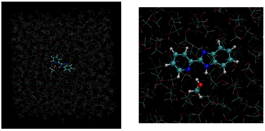
Figure 2. Illustration of the setup for excited-state QM/MM MD simulations. Left: overview of the full simulation box; Right: close-up view of the QM region and the surrounding solvent molecules.
The Q-Chem/Amber interface is driven by Amber (via the sander program), which calls Q-Chem to compute QM energies, forces, and electric field acting on MM atoms. Specifically, in our simulations, the forces for a given TD-DFT excited state (specified by CIS_STATE_DERIV) are computed at each timestep, along with the electric field generated by the QM region (i.e., the relaxed excited-state density and atomic nuclei) on MM atoms within the cutoff distance specified by qmcut under the &qmmm section. A simple script for running an interactive QM/MM simulation is shown below:
#!/bin/bash

export OMP_NUM_THREADS=16

export QCSCRATCH=$PWD

# Launch the S1 trajectory from snapshot #5500 from the S0 simulation

sander -O -i qmmm_md.in -o qmmm_md.out -p PBI_958methanol_40A.prmtop -c snap_5500.rst -r qmmm_md.rst -x qmmm_md.nc &
Note:
- One should ensure that the environment setup scripts for both Amber and Q-Chem have been loaded before running a simulation through the Q-Chem/Amber interface.
- It was found on some machines that the default
$QCSCRATCHlocation may not work properly for Q-Chem/Amber simulations. In such cases, setting$QCSCRATCHto be the current working directory ($PWD) would allow the simulation to run without crashing. - The value of
$OMP_NUM_THREADSshould be consistent with that ofnum_threadsas set in theqmmm_md.infile.
Below is an example SLURM script for running an excited-state QM/MM MD simulation using Q-Chem and Amber installed on a local cluster:
#!/bin/bash

#SBATCH --job-name=qmmm

#SBATCH --partition=LocalQ

#SBATCH --time=500:00:00

#SBATCH --ntasks=16

#SBATCH --error=qmmm.err


source /opt/qchem/6.3/qcenv.sh

source /opt/amber22/amber.sh

export OMP_NUM_THREADS=16

export QCSCRATCH=$PWD


sander -O \

  -i qmmm_md.in \

  -o qmmm_md.out \

  -p PBI_958methanol_40A.prmtop \

  -c snap_5500.rst \

  -r traj_1.rst \

  -x traj_1.nc